Getting environmental covariates for GFCR locations
covariates.RmdThis analysis extracts covariates for GFCR project sites from MERMAID, then combines that with coral cover data to plot the relationship between the two. In this example, the environmental data is maximum daily Sea Surface Temperature (SST) for a given number of days prior to the survey.
Get project data from MERMAID
The first step is to get coral cover data for GFCR projects from MERMAID. The following gets summary sample events, and then filters for projects whose tags contain “GFCR”, and projects that have hard coral cover data.
summary_sampleevents <- mermaid_get_summary_sampleevents()

gfcr_summary_sampleevents <- summary_sampleevents %>%
  filter(str_detect(tags, "GFCR")) %>%
  filter(!is.na(`benthicpit_percent_cover_benthic_category_avg_Hard coral`)) %>%
  rename(hard_coral_cover = `benthicpit_percent_cover_benthic_category_avg_Hard coral`)

gfcr_summary_sampleevents
## # A tibble: 142 × 383
## project_id project tags country site_id site latitude longitude reef_type
## <chr> <chr> <chr> <chr> <chr> <chr> <dbl> <dbl> <chr>
## 1 1370aaba-fe43-438e… Gulf o… Glob… Jordan 399b38… Aqab… 29.4 35.0 fringing
## 2 1370aaba-fe43-438e… Gulf o… Glob… Jordan 399b38… Aqab… 29.4 35.0 fringing
## 3 1370aaba-fe43-438e… Gulf o… Glob… Jordan 399b38… Aqab… 29.4 35.0 fringing
## 4 1370aaba-fe43-438e… Gulf o… Glob… Jordan 399b38… Aqab… 29.4 35.0 fringing
## 5 1370aaba-fe43-438e… Gulf o… Glob… Jordan 399b38… Aqab… 29.4 35.0 fringing
## 6 1370aaba-fe43-438e… Gulf o… Glob… Jordan 399b38… Aqab… 29.4 35.0 fringing
## 7 1370aaba-fe43-438e… Gulf o… Glob… Jordan 399b38… Aqab… 29.4 35.0 fringing
## 8 1370aaba-fe43-438e… Gulf o… Glob… Jordan 399b38… Aqab… 29.4 35.0 fringing
## 9 1370aaba-fe43-438e… Gulf o… Glob… Jordan 399b38… Aqab… 29.4 35.0 fringing
## 10 1370aaba-fe43-438e… Gulf o… Glob… Jordan 04e931… Nort… 29.5 35.0 fringing
## # ℹ 132 more rows
## # ℹ 374 more variables: reef_zone <chr>, reef_exposure <chr>, management_id <chr>,
## # management <chr>, management_est_year <int>, management_size <dbl>,
## # management_parties <chr>, management_compliance <chr>, management_rules <chr>,
## # sample_date <date>, data_policy_beltfish <chr>, data_policy_benthiclit <chr>,
## # data_policy_benthicpit <chr>, data_policy_benthicpqt <chr>,
## # data_policy_habitatcomplexity <chr>, data_policy_bleachingqc <chr>, …Summary of hard coral cover for projects
Summarise projects to show their tags, country, number of sites, and average hard coral cover.
gfcr_summary_sampleevents %>%
  group_by(project, tags, country) %>%
  summarise(
    n_sites = length(site),
    average_hard_coral_cover = mean(hard_coral_cover), .groups = "drop"
  )
## # A tibble: 7 × 5
## project tags country n_sites average_hard_coral_c…¹
## <chr> <chr> <chr> <int> <dbl>
## 1 Gulf of Aqaba Resilient Reefs Programme Glob… Jordan 29 21.4
## 2 Investing in Coral Reefs and the Blue E… Unit… Fiji 53 30.9
## 3 Maldives RREEF (GFCR) Glob… Maldiv… 11 43.4
## 4 SLCRI Bar Reef Seascape Inte… Sri La… 11 9.68
## 5 SLCRI Kayankerni Seascape Inte… Sri La… 11 44.4
## 6 SLCRI Pigeon Island Seascape Inte… Sri La… 7 55.9
## 7 Terumbu Karang Sehat Indonesia Program … Cons… Indone… 20 36.9
## # ℹ abbreviated name: ¹average_hard_coral_coverGet covariates for these sites
Next, get the relevant covariates for these sites.
List covariates
List available covariates.
## # A tibble: 19 × 11
##    title         description start_date end_date   license `sci:doi` keywords providers
##    <chr>         <chr>       <date>     <date>     <chr>   <chr>     <chr>    <list>
##  1 50 Reefs+ pr… This datas… 2026-02-22 2026-02-22 CC-BY-… 10.5281/… conserv… <tibble>
##  2 ACA Benthic … The Alan C… 2018-01-01 2021-01-01 propri… <NA>      ACA, Al… <tibble>
##  3 ACA Reef Ext… ACA reef e… 2026-01-01 2026-01-01 CC0 1.… <NA>      reef, r… <tibble>
##  4 Country Boun… This datas… 2024-10-04 2024-10-04 other   10.14284… adminis… <tibble>
##  5 Daily Global… NOAA Coral… 1985-03-25 2026-07-12 other   10.3390/… BAA, Bl… <tibble>
##  6 Daily Global… NOAA Coral… 1985-03-25 2026-07-12 other   10.3390/… coral b… <tibble>
##  7 Daily Global… NOAA Coral… 1985-01-01 2026-07-12 other   10.3390/… Coral R… <tibble>
##  8 Human popula… Coastal po… 2021-12-28 2021-12-28 MIT Li… 10.1111/… coastal… <tibble>
##  9 Marine Ecore… A biogeogr… 2011-11-18 2011-11-18 CC-BY-… 10.1641/… biodive… <tibble>
## 10 Market gravi… From econo… 2021-12-28 2021-12-28 MIT Li… 10.1111/… coral r… <tibble>
## 11 Number of po… Port locat… 2021-12-28 2021-12-28 MIT Li… 10.1111/… coral r… <tibble>
## 12 Tourism index Intensive … 2021-12-28 2021-12-28 MIT Li… 10.1111/… coral r… <tibble>
## 13 GPW Country … This datas… 2024-10-04 2024-10-04 other   10.14284… adminis… <tibble>
## 14 GPW Dispersa… Dispersal … 2026-01-01 2026-01-01 CC0 1.… <NA>      dispers… <tibble>
## 15 GPW Global S… Global Sed… 2000-01-01 2020-01-01 propri… <NA>      exposur… <tibble>
## 16 GPW Global S… Global sed… 2000-01-01 2020-01-01 CC0 1.… <NA>      gpw, se… <tibble>
## 17 GPW Land Use… Land Use a… 2000-01-01 2020-01-01 CC0-1.0 <NA>      land co… <tibble>
## 18 GPW MEOW Rea… Marine Eco… 2026-01-01 2026-01-01 cc-by-… <NA>      biodive… <tibble>
## 19 GPW Watershe… Watersheds… 2026-01-01 2026-01-01 CC0 1.… <NA>      gpw, hy… <tibble>
## # ℹ 3 more variables: `sci:citation` <chr>, bbox <list>, id <chr>
Get maximum SST for previous year
Focus on Sea Surface Temperature, and get the max for the 30 days prior to the survey data. Review the survey data:
gfcr_summary_sampleevents %>%
  distinct(project, site, latitude, longitude, sample_date)
## # A tibble: 142 × 5
## project site latitude longitude sample_date
## <chr> <chr> <dbl> <dbl> <date>
## 1 Gulf of Aqaba Resilient Reefs Programme Aqaba Marine… 29.4 35.0 2024-12-24
## 2 Gulf of Aqaba Resilient Reefs Programme Aqaba Marine… 29.4 35.0 2025-10-28
## 3 Gulf of Aqaba Resilient Reefs Programme Aqaba Marine… 29.4 35.0 2024-12-09
## 4 Gulf of Aqaba Resilient Reefs Programme Aqaba Marine… 29.4 35.0 2024-12-08
## 5 Gulf of Aqaba Resilient Reefs Programme Aqaba Marine… 29.4 35.0 2025-07-30
## 6 Gulf of Aqaba Resilient Reefs Programme Aqaba Marine… 29.4 35.0 2025-09-01
## 7 Gulf of Aqaba Resilient Reefs Programme Aqaba Marine… 29.4 35.0 2024-12-06
## 8 Gulf of Aqaba Resilient Reefs Programme Aqaba Marine… 29.4 35.0 2025-10-29
## 9 Gulf of Aqaba Resilient Reefs Programme Aqaba Marine… 29.4 35.0 2024-12-01
## 10 Gulf of Aqaba Resilient Reefs Programme Northern Dee… 29.5 35.0 2025-10-26
## # ℹ 132 more rowsWe can access daily SST data by using the function
get_zonal_statistics(), which takes the site latitude and
longitude, as well as the survey date, to find the data at that site for
n_days days prior, within the given radius,
and spatially aggregates it according to the specified
spatial_stat.
For example, to get the daily SST for each of the 30 days prior to (and including) the sample event, using the mean SST within 100m of the sites:
daily_sst <- gfcr_summary_sampleevents %>%
  get_zonal_statistics("Daily Global 5km Satellite Sea Surface Temperature (CoralTemp)", n_days = 30, radius = 100, spatial_stats = "mean")
Look at the returned data, keeping only the project information, site, survey date, hard coral cover, and zonal_statistics
daily_sst <- daily_sst %>%
  select(site, sample_date, hard_coral_cover, zonal_statistics)

daily_sst
## # A tibble: 142 × 4
## site sample_date hard_coral_cover zonal_statistics
## <chr> <date> <dbl> <list>
## 1 Sand Island Leeward 2023-05-24 38.5 <tibble [30 × 5]>
## 2 Sand Island South East 2023-05-24 38.2 <tibble [30 × 5]>
## 3 Elephant point East 2023-05-25 25.6 <tibble [30 × 5]>
## 4 Elephant point West 2023-05-25 15 <tibble [30 × 5]>
## 5 Sand Island North East 2023-05-25 63 <tibble [30 × 5]>
## 6 Pasikudah nearshore 2023-05-28 45.5 <tibble [30 × 5]>
## 7 Pasikudah offshore 2023-05-28 22.5 <tibble [30 × 5]>
## 8 Kalkudah 2023-05-29 46 <tibble [30 × 5]>
## 9 Pirate cove North to Headland 2023-06-14 73.5 <tibble [30 × 5]>
## 10 Pigeon island Landward - 01 2023-06-16 73.6 <tibble [30 × 5]>
## # ℹ 132 more rowsExpand zonal statistics
The zonal statistics are returned in a format that need to be expanded. Once they are, you can see they contain daily mean SST values:
daily_sst %>%
  unnest(zonal_statistics)
## # A tibble: 4,260 × 8
## site sample_date hard_coral_cover
## <chr> <date> <dbl>
## 1 Sand Island Leeward 2023-05-24 38.5
## 2 Sand Island Leeward 2023-05-24 38.5
## 3 Sand Island Leeward 2023-05-24 38.5
## 4 Sand Island Leeward 2023-05-24 38.5
## 5 Sand Island Leeward 2023-05-24 38.5
## 6 Sand Island Leeward 2023-05-24 38.5
## 7 Sand Island Leeward 2023-05-24 38.5
## 8 Sand Island Leeward 2023-05-24 38.5
## 9 Sand Island Leeward 2023-05-24 38.5
## 10 Sand Island Leeward 2023-05-24 38.5
## covariate date band
## <chr> <date> <dbl>
## 1 Daily Global 5km Satellite Sea Surface Temperature (CoralTemp) 2023-05-24 1
## 2 Daily Global 5km Satellite Sea Surface Temperature (CoralTemp) 2023-05-23 1
## 3 Daily Global 5km Satellite Sea Surface Temperature (CoralTemp) 2023-05-22 1
## 4 Daily Global 5km Satellite Sea Surface Temperature (CoralTemp) 2023-05-21 1
## 5 Daily Global 5km Satellite Sea Surface Temperature (CoralTemp) 2023-05-20 1
## 6 Daily Global 5km Satellite Sea Surface Temperature (CoralTemp) 2023-05-19 1
## 7 Daily Global 5km Satellite Sea Surface Temperature (CoralTemp) 2023-05-18 1
## 8 Daily Global 5km Satellite Sea Surface Temperature (CoralTemp) 2023-05-17 1
## 9 Daily Global 5km Satellite Sea Surface Temperature (CoralTemp) 2023-05-16 1
## 10 Daily Global 5km Satellite Sea Surface Temperature (CoralTemp) 2023-05-15 1
## spatial_stat value
## <chr> <dbl>
## 1 mean 30.6
## 2 mean 30.5
## 3 mean 30.5
## 4 mean 30.5
## 5 mean 30.5
## 6 mean 30.4
## 7 mean 30.1
## 8 mean 30.2
## 9 mean 30.0
## 10 mean 30.0
## # ℹ 4,250 more rowsSummarise zonal statistics
To get the maximum SST over the 30 day period, we use
summarise_zonal_statistics(), specifying that the temporal
statistic is the max:
max_sst <- daily_sst %>%
  summarise_zonal_statistics("max")

max_sst
## # A tibble: 142 × 5
## site sample_date hard_coral_cover zonal_statistics
## <chr> <date> <dbl> <list>
## 1 Sand Island Leeward 2023-05-24 38.5 <tibble [30 × 5]>
## 2 Sand Island South East 2023-05-24 38.2 <tibble [30 × 5]>
## 3 Elephant point East 2023-05-25 25.6 <tibble [30 × 5]>
## 4 Elephant point West 2023-05-25 15 <tibble [30 × 5]>
## 5 Sand Island North East 2023-05-25 63 <tibble [30 × 5]>
## 6 Pasikudah nearshore 2023-05-28 45.5 <tibble [30 × 5]>
## 7 Pasikudah offshore 2023-05-28 22.5 <tibble [30 × 5]>
## 8 Kalkudah 2023-05-29 46 <tibble [30 × 5]>
## 9 Pirate cove North to Headland 2023-06-14 73.5 <tibble [30 × 5]>
## 10 Pigeon island Landward - 01 2023-06-16 73.6 <tibble [30 × 5]>
## summary_zonal_statistics
## <list>
## 1 <tibble [1 × 8]>
## 2 <tibble [1 × 8]>
## 3 <tibble [1 × 8]>
## 4 <tibble [1 × 8]>
## 5 <tibble [1 × 8]>
## 6 <tibble [1 × 8]>
## 7 <tibble [1 × 8]>
## 8 <tibble [1 × 8]>
## 9 <tibble [1 × 8]>
## 10 <tibble [1 × 8]>
## # ℹ 132 more rowsThe original zonal statistics are returned along with the summarised zonal statistics, which we expand. Now, we only have one value for each sample event – the maximum SST. This is returned along with the start and end date of the covariate data used, as well as the number of dates. This is useful information cases where the covariate data may not be available for all requested dates.
## # A tibble: 142 × 11
##    site                          sample_date hard_coral_cover
##    <chr>                         <date>                 <dbl>
##  1 Sand Island Leeward           2023-05-24              38.5
##  2 Sand Island South East        2023-05-24              38.2
##  3 Elephant point East           2023-05-25              25.6
##  4 Elephant point West           2023-05-25              15
##  5 Sand Island North East        2023-05-25              63
##  6 Pasikudah nearshore           2023-05-28              45.5
##  7 Pasikudah offshore            2023-05-28              22.5
##  8 Kalkudah                      2023-05-29              46
##  9 Pirate cove North to Headland 2023-06-14              73.5
## 10 Pigeon island Landward - 01   2023-06-16              73.6
##    covariate                                                      start_date end_date
##    <chr>                                                          <date>     <date>
##  1 Daily Global 5km Satellite Sea Surface Temperature (CoralTemp) 2023-04-25 2023-05-24
##  2 Daily Global 5km Satellite Sea Surface Temperature (CoralTemp) 2023-04-25 2023-05-24
##  3 Daily Global 5km Satellite Sea Surface Temperature (CoralTemp) 2023-04-26 2023-05-25
##  4 Daily Global 5km Satellite Sea Surface Temperature (CoralTemp) 2023-04-26 2023-05-25
##  5 Daily Global 5km Satellite Sea Surface Temperature (CoralTemp) 2023-04-26 2023-05-25
##  6 Daily Global 5km Satellite Sea Surface Temperature (CoralTemp) 2023-04-29 2023-05-28
##  7 Daily Global 5km Satellite Sea Surface Temperature (CoralTemp) 2023-04-29 2023-05-28
##  8 Daily Global 5km Satellite Sea Surface Temperature (CoralTemp) 2023-04-30 2023-05-29
##  9 Daily Global 5km Satellite Sea Surface Temperature (CoralTemp) 2023-05-16 2023-06-14
## 10 Daily Global 5km Satellite Sea Surface Temperature (CoralTemp) 2023-05-18 2023-06-16
##    n_dates  band spatial_stat temporal_stat value
##      <dbl> <dbl> <chr>        <chr>         <dbl>
##  1      30     1 mean         max            30.6
##  2      30     1 mean         max            30.6
##  3      30     1 mean         max            30.6
##  4      30     1 mean         max            30.6
##  5      30     1 mean         max            30.6
##  6      30     1 mean         max            30.7
##  7      30     1 mean         max            30.7
##  8      30     1 mean         max            30.7
##  9      30     1 mean         max            30.2
## 10      30     1 mean         max            30.3
## # ℹ 132 more rows
Visualize
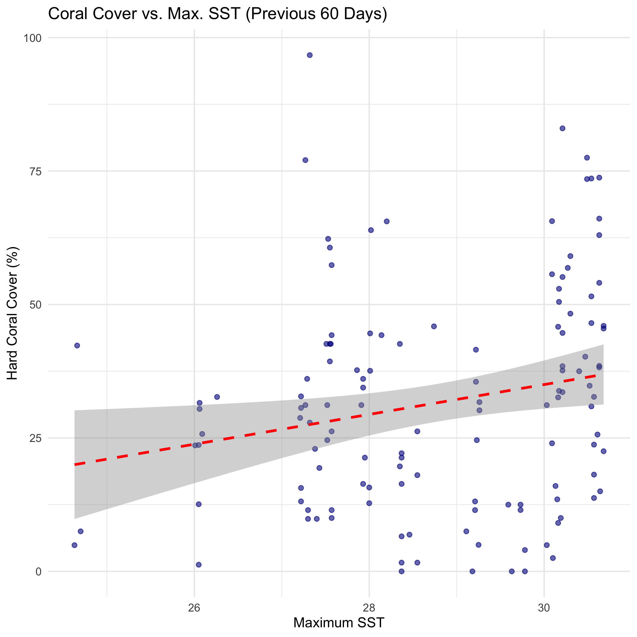
Finally, visualize coral cover against the maximum Sea Surface Temperature for the past 30 days.
ggplot(
  max_sst,
  aes(
    x = value,
    y = hard_coral_cover
  )
) +
  geom_point(color = "darkblue", alpha = 0.6) +
  geom_smooth(method = "lm", color = "red", linetype = "dashed") +
  labs(
    title = paste("Coral Cover vs. Max. SST (Previous 30 Days)"),
    x = "Maximum SST",
    y = "Hard Coral Cover (%)"
  ) +
  theme_minimal()